Benchmarks
External and internal benchmarks for `monoprop`.
Comparison with other packages
We provide standalone benchmark scripts comparing monoprop against other open-source
Majorana and Pauli propagation engines. The benchmark suite includes memory and time
performance metrics, providing insights into the efficiency of different
propagation engines.
You can find the benchmark scripts in the benches/third_party directory.
The scripts are designed to be run in a controlled environment,
ensuring fair comparisons between different engines.
Majorana Propagation
The chosen problem is the 1D Hubbard model, tracking the runtime, expectation value, and operator size at each Trotter step.
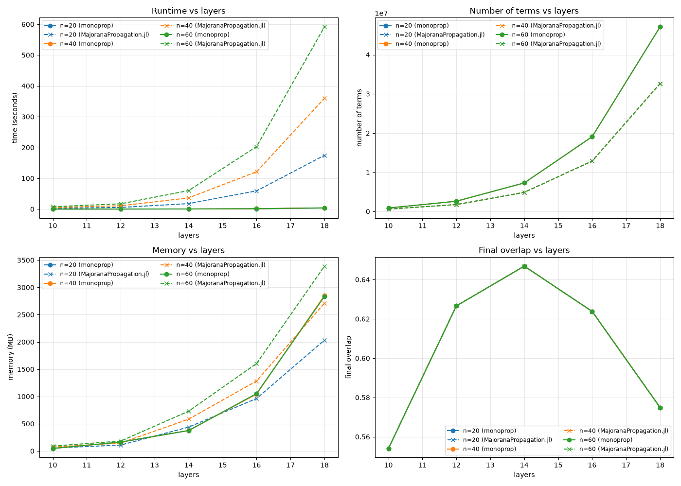
Number of terms, final overlap, runtime, and memory vs. circuit layers for the 1D Fermi-Hubbard
model, comparing monoprop against MajoranaPropagation.jl. See the
section below for details on the setup and how to reproduce these results.
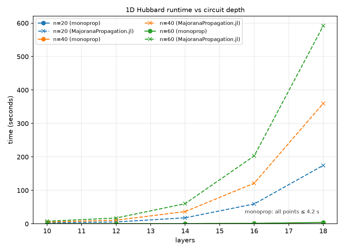
Runtime on its own, both axes linear. Solid lines are monoprop, dashed are
MajoranaPropagation.jl, and colour is the system size. Read it as seconds: the Julia engine's
591 s at 60 sites / 18 layers is drawn 140× the height of monoprop's 4.2 s, and all three
monoprop curves consequently lie along the bottom of the axis — annotated with the top of that
band, since flat here means small, not zero. For monoprop's own growth with depth, read the
term-count and memory panels of the combined figure, or the numbers below.
SPECS
The benchmark is run on Leonardo (CINECA), one exclusive DCGP node per engine:
- CPU: 2× Intel Xeon Platinum 8480+ (112 cores total, Sapphire Rapids)
- RAM: ~480 GB
Each engine runs at the thread count it is fastest at — monoprop at 56 threads,
MajoranaPropagation.jl at 28 — since they do not peak at the same count.
The end-to-end workflow is:
- Set up the Python environment.
- Install Julia and
MajoranaPropagation.jl. - Run the benchmarks to produce the JSONL result files.
- Plot the results to produce
majorana_results.pngandmajorana_runtime.png.
1. Set up the Python environment
# Navigate to this directory
cd benches/third_party

# Create the venv and install all Python dependencies (including monoprop itself, in editable mode)
uv sync
This installs monoprop and numpy.
2. Install Julia and MajoranaPropagation.jl
You can find the installation instructions for Julia and MajoranaPropagation.jl in the official documentation.
# Install juliaup and the latest stable Julia release
curl -fsSL https://install.julialang.org | sh
Once Julia has been installed, you can install and instantiate the required packages for the benchmark:
julia --project=@. -e 'using Pkg; Pkg.instantiate()'
Then, you can precompile the MajoranaPropagation.jl package to ensure that it is ready for use:
julia --project=@. -e 'using Pkg; Pkg.precompile()'3. Run the benchmarks
You can run the benchmarks using the provided bash script for both Python and Julia engines. The script will execute the benchmarks and generate the results in two separate JSON files: julia_hubbard1d_benchmark_results.jsonl for the Julia engine and monoprop_hubbard1d_benchmark_results.jsonl for the Python engine.
# Run the benchmarks for both Python and Julia engines
bash run_benchmarks.sh
Each line of both JSONL files is one benchmark run (one system size / circuit depth pair), with:
n_spinful_sites: number of spinful sites in the 1D Hubbard chain.n_layers: number of Trotter layers simulated.num_terms: number of Majorana terms kept in the operator at the final layer.final_overlap: expectation value at the final layer.runtime_seconds: wall-clock time to run alln_layerslayers.memory_MB: operator memory footprint at the final layer, in megabytes.num_threads: thread count the run was given (monoprop_NUM_THREADS/JULIA_NUM_THREADS).cpu_seconds: CPU time consumed over the timed loop, summed over all threads.busy_cores:cpu_seconds / runtime_seconds— how many cores the run actually kept busy. A value near 1 means the run was serial, irrespective ofnum_threads.peak_rss_MB,library_version,host: provenance for the row.
Both engines are multithreaded, but they do not peak at the same thread count, so
run_benchmarks.sh reads monoprop_NUM_THREADS and JULIA_NUM_THREADS from the environment
(default 8 each) rather than fixing them. The Julia results additionally record container and
gc_seconds: only VectorMajoranaSum dispatches into MajoranaPropagation.jl's
AcceleratedKernels path, while the dict-backed MajoranaSum is serial regardless of thread count.
The Python results additionally record affinity_cores and mu_gates (see --mu-gates, which
restores the inert chemical-potential gates that the Julia circuit does not have).
4. Plot the results
uv run python plot_results.pyThis reads the json file results for each simulation and produces two images: majorana_results.png,
combining four linear scale panels (number of terms, final overlap, runtime, and memory) in a 2x2
grid, and majorana_runtime.png, the runtime alone on linear axes. Runtime gets its own file
because it is the quantity cited on its own.
Results
Number of terms, final-state overlap, runtime, and memory footprint versus circuit depth for the
1D Hubbard model, comparing monoprop against MajoranaPropagation.jl across system sizes
n=20, 40, and 60. Final overlaps agree to within 1.8e-6, confirming both engines simulate
the same physics, and monoprop keeps 1.44-1.50× more terms at equal atol and cutoff.
monoprop is 22-142× faster over the grid, and the gap widens with both depth and system size:
21.9× at 20 sites / 10 layers, 141.6× at 60 sites / 18 layers (4.2 s versus 592 s). Its runtime
is nearly flat in site count while the Julia engine's grows roughly linearly. Dividing out the
cores each engine actually kept busy leaves 8.5-52×, so the majority of the gap is algorithmic
rather than a thread-count artifact. Memory is comparable at low depth and diverges in
monoprop's favour as the operator grows (2834 MB versus 3390 MB at 60 sites / 18 layers).
Pauli Propagation
The chosen problem is the Trotterized time evolution of a 2D transverse-field Ising model (TFIM), tracking the runtime, expectation value, and operator size at each Trotter step.
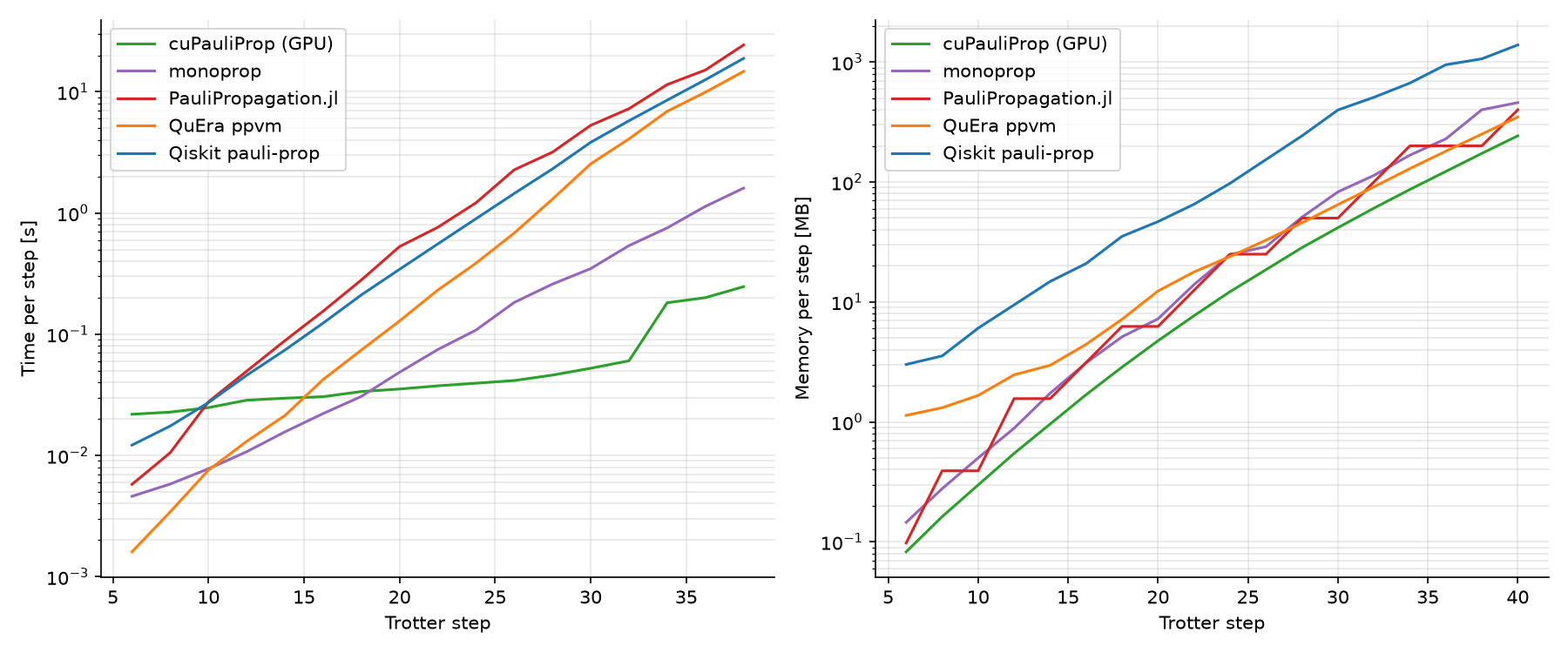
Runtime and memory usage per Trotter step for the 2D TFIM problem, comparing monoprop against
other Pauli propagation engines. See the Pauli Propagation section below for
details on the setup and how to reproduce these results.
SPECS
- CPU: AMD Ryzen Threadripper PRO 7955WX 16-Cores
- RAM: 128 GB in dual channel
- GPU: Nvidia RTX 5090 with 32 GB VRAM
The end-to-end workflow is:
- Choose the simulation settings in
settings.json. - Set up the Python environment.
- (Optional) install Julia and
PauliPropagation.jl. - Run the benchmarks to produce
results.json. - Plot the results to produce
results.png.
1. Choose the simulation settings
All simulation parameters live in settings.json and are shared by every engine
(Python and Julia alike), so a single edit compares them all on an identical problem instance:
| Key | Meaning |
|---|---|
nx, ny | Size of the qubit grid (columns × rows); total qubits = nx * ny, row-major indexed. |
hx | Transverse (X) field strength. |
hz | Longitudinal (Z) field strength, i.e. the Hamiltonian's tilt. |
j | ZZ coupling strength between nearest-neighbor qubits. |
dt | Trotter step size. |
step_min | First Trotter step to simulate (inclusive). |
step_max | Last Trotter step to simulate (inclusive). |
lower_atol | Coefficient magnitude below which Pauli terms are truncated. |
cutoff | Maximum Pauli weight to keep during propagation; null disables weight truncation. |
obs_qubits | The qubit pair (row-major grid index) whose ZZ correlator is measured. |
Edit the values directly in settings.json before running the benchmarks — e.g. increase
nx/ny for a larger system, widen step_min/step_max to simulate more Trotter steps, or
relax lower_atol/cutoff to trade accuracy for speed. All engines read this same file, so no
code changes are needed to reproduce a benchmark under different conditions.
Qiskit pauli-prop is the one exception: its propagate_through_circuit API has no weight-based
cutoff, only a mandatory positive max_terms (which also caps its memory pre-allocation, so it
can't be left unbounded). run_model.py sets it to monoprop's own term count at each step, so its
per-step term budget tracks cutoff/lower_atol indirectly through monoprop rather than directly.
2. Set up the Python environment
# Navigate to this directory
cd benches/third_party

# Create the venv and install all Python dependencies (including monoprop itself, in editable mode)
uv sync
This installs monoprop, qiskit, ppvm, pauli-prop, and cuquantum-python-cu12. Running the
cuPauliProp (GPU) engine requires an NVIDIA GPU with a working CUDA setup; the other three Python
engines (monoprop, QuEra ppvm, Qiskit pauli-prop) run on CPU only.
3. (Optional) install Julia and PauliPropagation.jl
Skip this step if you only want to compare the Python engines — run_model.py and
plot_results.py work fine without it. Install it if you also want the PauliPropagation.jl
comparison:
# Install juliaup and the latest stable Julia release
curl -fsSL https://install.julialang.org | sh
Once Julia has been installed, add some utils:
julia -e 'using Pkg; Pkg.add(["JSON", "ProgressMeter"])'Finally, install the package PauliPropagation.jl v0.7.3:
julia -e 'using Pkg; Pkg.add(Pkg.PackageSpec(name="PauliPropagation", version="0.7.3"))'4. Run the benchmarks
# Run the Python engines (monoprop, QuEra ppvm, Qiskit pauli-prop, cuPauliProp) — (re)writes results.json from scratch
uv run python run_model.py

# (Optional) run the Julia engine — merges its results into the existing results.json
julia run_model.jl
run_model.py must be run first: it (re)creates results.json from settings.json.
run_model.jl then reads that file and adds the PauliPropagation.jl entries to it, so
re-running run_model.py afterwards overwrites the file and drops them again — rerun
run_model.jl too if you do.
For every engine, results.json collects, indexed by Trotter step:
num_terms: the number of Pauli/Majorana terms kept in the evolving operator, for every step.runtime: wall-clock time per step, in seconds. The first step is excluded: it carries each engine's warm-up (JIT compilation, first-touch allocation), which is not what the per-step comparison is measuring.memory: the memory footprint of the evolving operator, in megabytes, for every step. Where an engine exposes its own accounting this is exact (monoprop's C++ operator-memory accounting, cuPauliProp's cupy device memory pool,PauliPropagation.jl'sBase.summarysizeof the Pauli sum);QuEra ppvmandQiskit pauli-propexpose no such accounting, so their footprint is reconstructed by accumulating this process's host-memory growth across each of their own steps.expvals: theZZexpectation value onobs_qubits, for every step.
5. Plot the results
uv run python plot_results.pyThis reads results.json and produces a single image, pauli_results.png, combining two log-scale
panels (runtime per Trotter step and operator memory footprint per Trotter step) side by side, for
each engine present in the file (so they reflect whichever engines you actually ran in step 4).
Results
Runtime and memory footprint per Trotter step for the 2D TFIM problem above, comparing
monoprop against cuPauliProp (GPU), PauliPropagation.jl, QuEra ppvm, and Qiskit pauli-prop. monoprop tracks the GPU-accelerated cuPauliProp closely while running on CPU,
and outperforms all other CPU-only engines in both time and memory as the operator grows.
Scaling with lattice size
The benchmark above fixes the lattice at 6x6 and walks the Trotter steps. The second Pauli benchmark does the opposite: it holds the circuit depth and the truncation fixed and grows the lattice, from 6x6 (36 qubits) to 18x18 (324 qubits). Every engine runs the identical model at each size, in its own subprocess, and contributes one totals record per size.
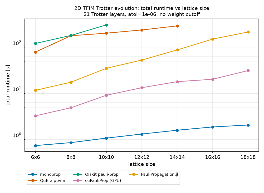
At a fixed coefficient truncation the operator saturates: past ~100 qubits every engine carries
the same ~5.8M terms whatever the lattice, so this measures cost per term kept rather than a
growing problem. monoprop's total runtime stays nearly flat in that regime, which is what makes
the gap widen with size.
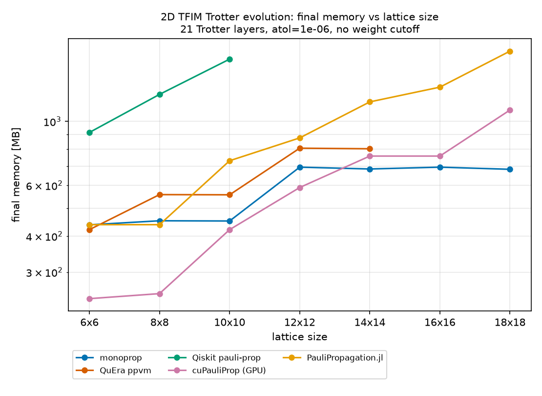
The same saturation shows up in memory: monoprop's footprint flattens near 690 MB from 12x12
on, while PauliPropagation.jl's keeps climbing to ~1.8 GB at 324 qubits. Compare across engines
only with the third caveat below in mind — these are not all the same measurement.
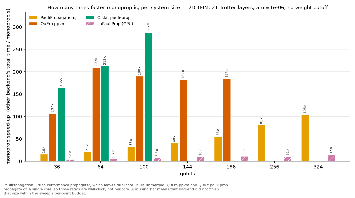
| qubits | PauliPropagation.jl | QuEra ppvm | Qiskit pauli-prop | cuPauliProp (GPU) |
|---|---|---|---|---|
| 36 | 16× | 107× | 165× | 4.4× |
| 64 | 21× | 209× | 213× | 5.7× |
| 100 | 33× | 190× | 287× | 8.5× |
| 144 | 40× | 182× | – | 10× |
| 196 | 55× | 184× | – | 11× |
| 256 | 81× | – | – | 11× |
| 324 | 105× | – | – | 15× |
A dash means the engine did not finish that size within the 300 s per-point budget. Three caveats belong with these ratios:
- Only two of the four CPU engines use more than one core.
QuEra ppvmand Qiskit'spauli-proppropagate on a single core — measured at 0.99 busy cores mid-propagation — and no environment variable changes it: ppvm's rayon-parallelPauliSumlives in itsconfig::dashmapvariant while its Python bindings expose only theindexmapone, and Qiskit's_accelerateextension contains no parallel path at all. The ratios above are therefore wall-clock, not per-core. PauliPropagation.jlruns in its fastest documented configuration, theVectorPauliSumcontainer driven byPerformance.propagate!, which needs the dev branch (0.8.0+) for thePerformancesubmodule. That path leaves duplicate Pauli strings unmerged, so it reports ~38% more terms than the exactpropagatepath and its expectation value differs by ~1e-4 — its term count is a storage count, not an operator size.- The memory figure is not one quantity.
monopropandcuPauliPropreport their own operator accounting,PauliPropagation.jlitsBase.summarysize, and ppvm and Qiskit only a process-RSS proxy, because they expose nothing else.
SPECS
The benchmark is run on Leonardo (CINECA):
- CPU: 2× Intel Xeon Platinum 8480+ (112 cores total) —
monopropat 56 threads,PauliPropagation.jlat 28 threads. - GPU: 1× NVIDIA A100 with 64 GB HBM2e, for
cuPauliProp.
Each record in the committed data carries its own host, threads and library_version, and
both plotting scripts print that provenance beside the numbers.
Running it
cd benches/third_party/pauli_prop

# Redraw both figures from the committed ladder — seconds, no propagation
uv run python plot_scaling.py scaling_results.jsonl
uv run python plot_speedup.py scaling_results.jsonl

# Or measure it: one subprocess per (size, engine), 5 minutes per point
uv run python run_scaling.py --output results/scaling.jsonl --timeout 300 \
  --threads monoprop=56 juliapp=28
Two build notes: 324 qubits needs a monoprop mode tier at least that large
(-Dmonoprop_MAX_NUM_MODES=352, since tiers come in 32-mode blocks), and the Julia engine here
needs the dev branch — Pkg.add(url="https://github.com/SparqleSim/PauliPropagation.jl", rev="dev") — while the fixed-size run_model.jl above is fine on the pinned v0.7.3.
Internal benchmarks
The monoprop repository includes a pytest suite measuring the time and
peak resident memory (RSS) of monoprop's core operations.
The suite is separated from the test suite and can be run with just bench.
See below for more detailed instructions.
Running
Each run takes a label and becomes one column in results/REPORT.md, so
serial, MPI, and thread variants sit side by side. Extra args go to pytest.
uv sync --group bench                          # once

just bench serial                              # serial run, column "serial"
just bench-smoke                               # quick sanity check (tiny sizes)
just bench serial --num-modes 64 --bench-rounds 10

monoprop_NUM_THREADS=10 just bench serial-t10  # cap the partition count

uv run --group bench python benches/report.py  # rebuild report, no re-run
MPI
Communicator-aware: operations are barrier-wrapped so the timed cost is the makespan across ranks, and memory is the peak of the RSS summed across ranks (shared pages counted per rank, so an upper bound), not the sum of per-rank peaks.
just bench-build-mpi                           # build once (MPI on)
monoprop_NUM_THREADS=2 just bench-mpi r5t2 5 --map-by slot:PE=2 --bind-to core
The MPI build must stay loaded. monoprop builds MPI=OFF by default; a
non-MPI extension ignores the communicator, so every rank holds the full
operator (N× memory). The recipes use --no-sync so the MPI build survives —
rebuild after editing sources. just bench-mpi checks monoprop.has_mpi and
aborts if MPI is missing; extra args are forwarded to mpiexec (as root, add
--allow-run-as-root).
Benchmarks
Random (bench_random.py; configurable, both pictures) — build_graph,
pare, energy, gradient (graph-based), and inplace. CLI options:
| Option | Meaning | Default |
|---|---|---|
--gen-length | Majorana operators per generator | 4 |
--obs-terms | observable terms | 10000 |
--num-generators | generators (circuit gates) | 100 |
--num-modes | fermionic modes (Majorana indices = 2·modes) | 128 |
--cutoff | truncation cutoff | 6 |
--seed | RNG seed | 0 |
--bench-rounds | fixed timing rounds (MPI-safe) | 1 |
Models (bench_models.py; fixed, in-place, slow):
test_model[hubbard]— 120-qubit Fermi-Hubbard, 29-step Trotter.test_model[pauli]— 127-qubit Pauli-basis kicked-Ising, 20 layers.
Override any config field via --<model>-<field> (e.g. --pauli-num-layers 30);
just bench --help lists all.
Output
Each run writes results/time-<label>.json (pytest-benchmark) and
<label>.json (everything else); report.py merges all labels into
results/REPORT.md.